Data Wrangling

Reading Files

Project Management

• Important to understand your file structure and where you save everything
• Working directory
• “Default location where R will look for files you want to load and where it will put any files you save” source

#Returns the file path of the current working directory
getwd()

#Set Working Directory
setwd()

• Easiest way to set Working Directory:
  • Session -> Set Working Directory -> Choose Directory
  • Point and Click Method

Excel

Data Files in Excel

• Formats .xls and .csv - what’s the difference?

• File extensions .xls and .xlsx are proprietary Excel formats, binary files

• csv is an extension for Comma Separated Value files. They are text files - directly readable.

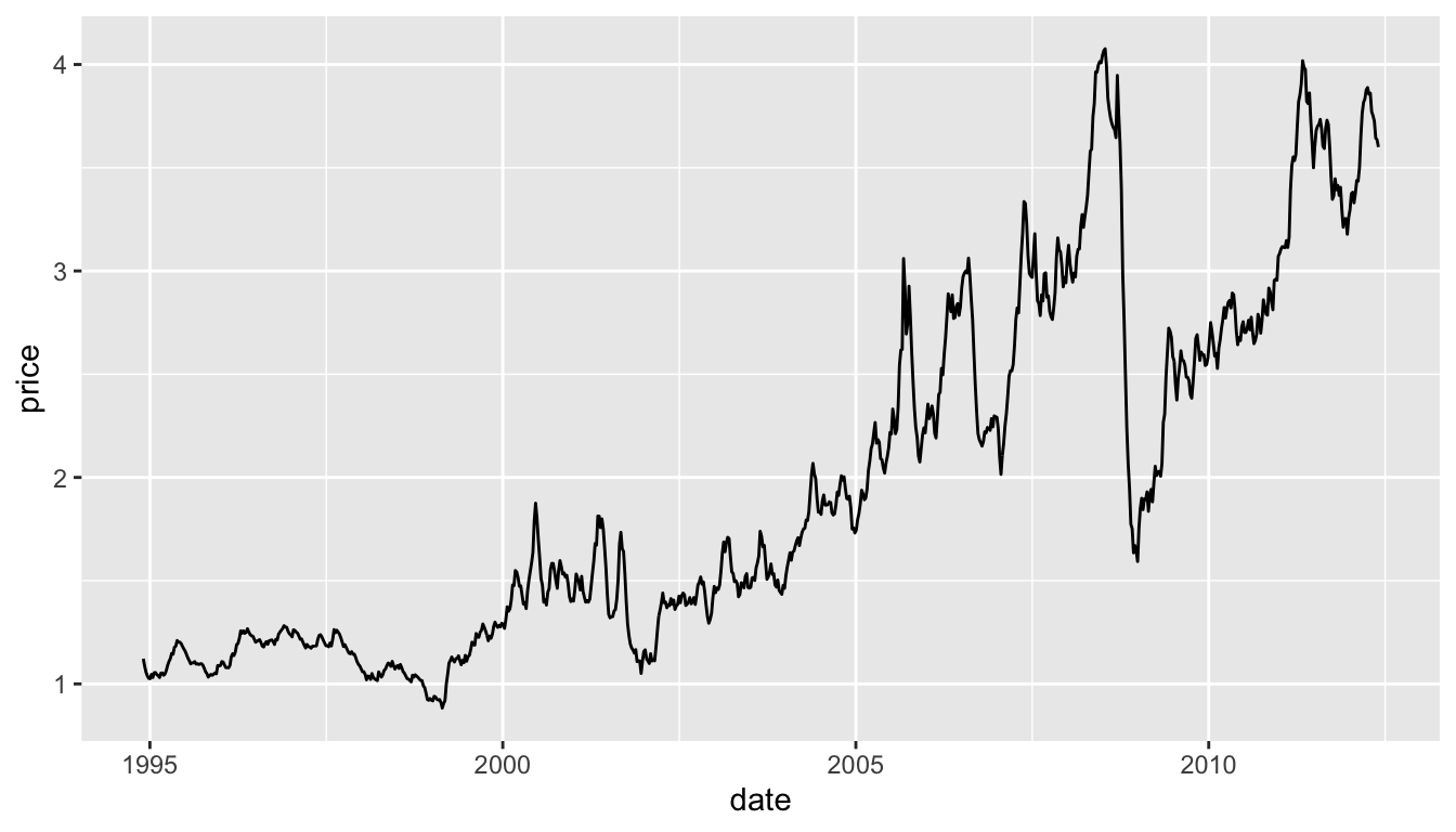
• Motivating Example: Gas prices in the Midwest since 1994

CSV - comma-separated values (contains plain text entries and commas) XLS - specific spreadsheet file for Microsoft Excel. Can’t be opened with a text editor

MOTIVATING EXAMPLE

Gas Prices in the Midwest

Year-Month	Week 1	…3	Week 2	…5	Week 3	…7	Week 4	…9	Week 5	…11
NA	End Date	Value	End Date	Value	End Date	Value	End Date	Value	End Date	Value
1994-Nov	NA	NA	NA	NA	NA	NA	28-Nov	1.122	NA	NA
1994-Dec	5-Dec	1.086	12-Dec	1.057	19-Dec	1.039	26-Dec	1.027	NA	NA
1995-Jan	2-Jan	1.025	9-Jan	1.046	16-Jan	1.031	23-Jan	1.054	30-Jan	1.055
1995-Feb	6-Feb	1.045	13-Feb	1.04	20-Feb	1.031	27-Feb	1.052	NA	NA
1995-Mar	6-Mar	1.053	13-Mar	1.042	20-Mar	1.048	27-Mar	1.065	NA	NA

What’s the difference read_csv vs. read_* ??

read_csv is just one way to read a file using the readr package:

• read_delim: the most generic function. Use the delim argument to read a file with any type of delimiter
• read_tsv: read tab separated files
• read_lines: read a file into a vector that has one element per line of the file
• read_file: read a file into a single character element
• read_table: read a file separated by space

Start by having them load tidyverse. (Includes all of the packages we’ll be using today)

Your Turn

Have a look at the parameters of read_csv to solve the following problems:

1. Read the first two lines of the file into an object called midwest_names

2. Read everything EXCEPT the first two lines into an object called midwest_data

Hint: Visit http://unl-statistics.github.io/R-workshops/r-format/data/midwest.csv to download the data into your current working directory (getwd()) and look at it in Excel to help figure out what the issue is.

Your Turn Solutions

midwest_names <- read_csv(
"midwest.csv", 
  n_max= 2, col_names = FALSE)


midwest_data <- read_csv(
"midwest.csv", 
  skip = 2, col_names = FALSE)

Quick Lesson in Data Cleaning

library(lubridate) # works with dates
library(tidyverse)
values <- c(midwest_data$X3, midwest_data$X5, midwest_data$X7, 
            midwest_data$X9, midwest_data$X11)
dates <- c(paste(midwest_data$X1, midwest_data$X2, sep = "-"), 
           paste(midwest_data$X1, midwest_data$X4, sep = "-"),
           paste(midwest_data$X1, midwest_data$X6, sep = "-"),
           paste(midwest_data$X1, midwest_data$X8, sep = "-"),
           paste(midwest_data$X1, midwest_data$X10, sep = "-"))

dates <- dates[!is.na(values)] #removing NAs
values <- values[!is.na(values)] #removing Nas

dates <- ymd(dates)

midwest_gas <- data_frame(date = dates, price = values)
midwest_gas <- arrange(midwest_gas, dates)

explain - paste function values - vector of the different columns dates - vector of different dates (combining year/month with month/day)

ymd function - transforms dates stored in a character to date with year, month, day components

Now we can make a plot!

library(ggplot2)

ggplot(midwest_gas, aes(x = date, y = price)) + geom_line()

Reading Excel Data

Download the midwest.xls file to your current working directory (getwd())

library(readxl)
midwest2 <- read_excel("https://github.com/unl-statistics/R-workshops/raw/main/r-format/data/midwest.xls") 
head(midwest2)

Something isn’t quite right here…

Year-Month	Week 1	...3	Week 2	...5	Week 3	...7	Week 4	...9	Week 5	...11
NA	End Date	Value	End Date	Value	End Date	Value	End Date	Value	End Date	Value
1994-Nov	NA	NA	NA	NA	NA	NA	39779	1.1220000000000001	NA	NA
1994-Dec	39786	1.0860000000000001	39793	1.0569999999999999	39800	1.0389999999999999	39807	1.0269999999999999	NA	NA

Reading Excel Data: Attempt #2

The 2nd row of the excel file also contains variable names.

Let’s skip the first this time. We can then rename the first column.

midwest2 <- read_excel("https://github.com/unl-statistics/R-workshops/raw/main/r-format/data/midwest.xls", skip = 1) #<<
names(midwest2)[1] <- "Year-Month"
head(midwest2)

Year-Month	End Date...2	Value...3	End Date...4	Value...5	End Date...6	Value...7	End Date...8	Value...9	End Date...10	Value...11
1994-Nov	NA	NA	NA	NA	NA	NA	2012-11-28	1.122	NA	NA
1994-Dec	2012-12-05	1.086	2012-12-12	1.057	2012-12-19	1.039	2012-12-26	1.027	NA	NA
1995-Jan	2012-01-02	1.025	2012-01-09	1.046	2012-01-16	1.031	2012-01-23	1.054	2012-01-30	1.055

Better, but not yet perfect…

How can you fix this? Brute force way by renaming all columns? Take this into consideration when entering in your data into spreadsheets (no merged columns names with subheadings)

Other Data Types

haven Package

• Other file formats can be read using the functions from package haven

• SPSS: read_spss

• SAS: read_xpt

• Stata: read_dta

Useful Packages for Other Data Files

• foreign package reads from Minitab, Systat, etc. files.

• rgdal package reads shapefiles (for maps)

• sf package reads arcgis files, etc. sf package

R knowledge Spatial, by Allison Horst

Your Turn (~2 minutes)

The NHANES (National Health and Nutrition Survey) publishes data in the SAS xport format:

https://wwwn.cdc.gov/Nchs/Nhanes/continuousnhanes/default.aspx?BeginYear=2013

1. Scroll to the bottom, choose one of the datasets (Demographics, Examination, etc.). Download the Data file (XPT)

2. Use read_xpt() to load the file into R

3. Briefly examine the dataset you’ve imported (use head or tail, etc)

Solution

library(haven) 
sas.data <- read_xpt("../data/DEMO_G.XPT")
sas.data %>% head(2)

# A tibble: 2 × 48
   SEQN SDDSRVYR RIDSTATR RIAGENDR RIDAGEYR RIDAGEMN RIDRETH1 RIDRETH3 RIDEXMON
  <dbl>    <dbl>    <dbl>    <dbl>    <dbl>    <dbl>    <dbl>    <dbl>    <dbl>
1 62161        7        2        1       22       NA        3        3        2
2 62162        7        2        2        3       NA        1        1        1
# ℹ 39 more variables: RIDEXAGY <dbl>, RIDEXAGM <dbl>, DMQMILIZ <dbl>,
#   DMQADFC <dbl>, DMDBORN4 <dbl>, DMDCITZN <dbl>, DMDYRSUS <dbl>,
#   DMDEDUC3 <dbl>, DMDEDUC2 <dbl>, DMDMARTL <dbl>, RIDEXPRG <dbl>,
#   SIALANG <dbl>, SIAPROXY <dbl>, SIAINTRP <dbl>, FIALANG <dbl>,
#   FIAPROXY <dbl>, FIAINTRP <dbl>, MIALANG <dbl>, MIAPROXY <dbl>,
#   MIAINTRP <dbl>, AIALANGA <dbl>, WTINT2YR <dbl>, WTMEC2YR <dbl>,
#   SDMVPSU <dbl>, SDMVSTRA <dbl>, INDHHIN2 <dbl>, INDFMIN2 <dbl>, …