Data Wrangling

Using dplyr

Data Wrangling Cheat Sheet, by RStudio

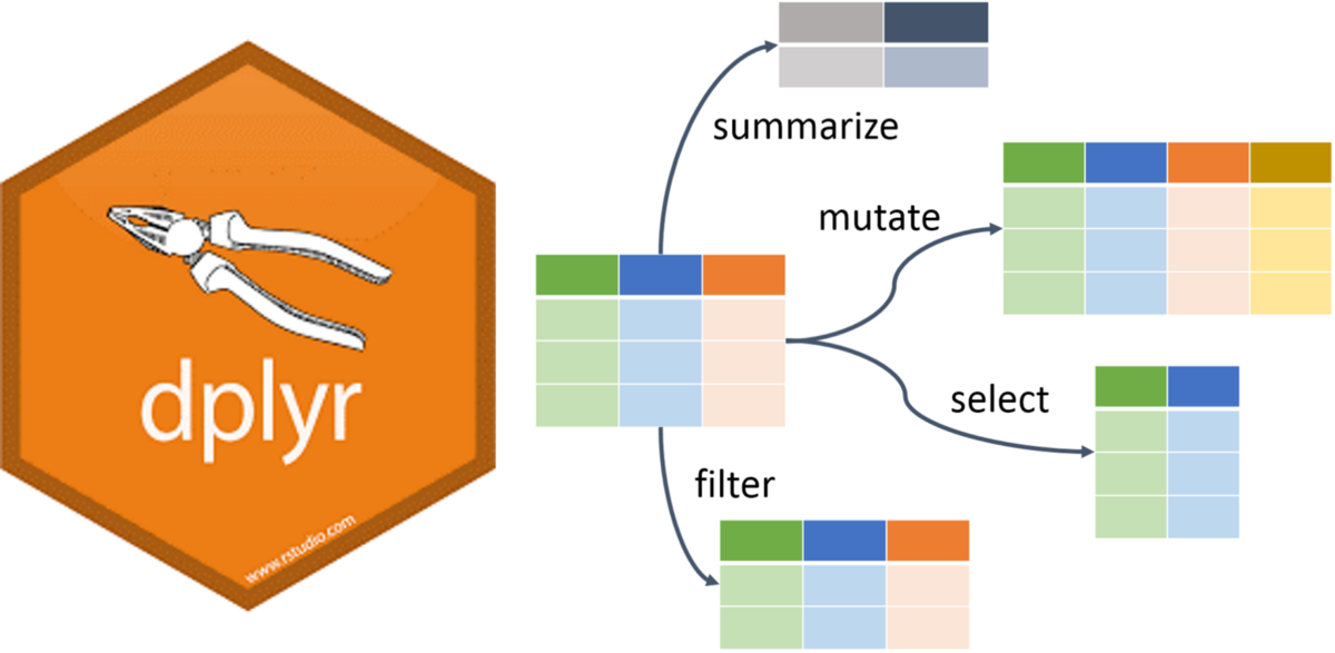
dplyr terminology

There are some of the primary dplyr verbs, representing distinct data analysis tasks:

Filter: Select specified rows of a data frame, produce subsets
Arrange: Reorder the rows of a data frame
Select: Select particular columns of a data frame
Mutate: Add new or change existing columns of the data frame (as functions of existing columns)
Summarise: Create collapsed summaries of a data frame
Group By: Introduce structure to a data frame

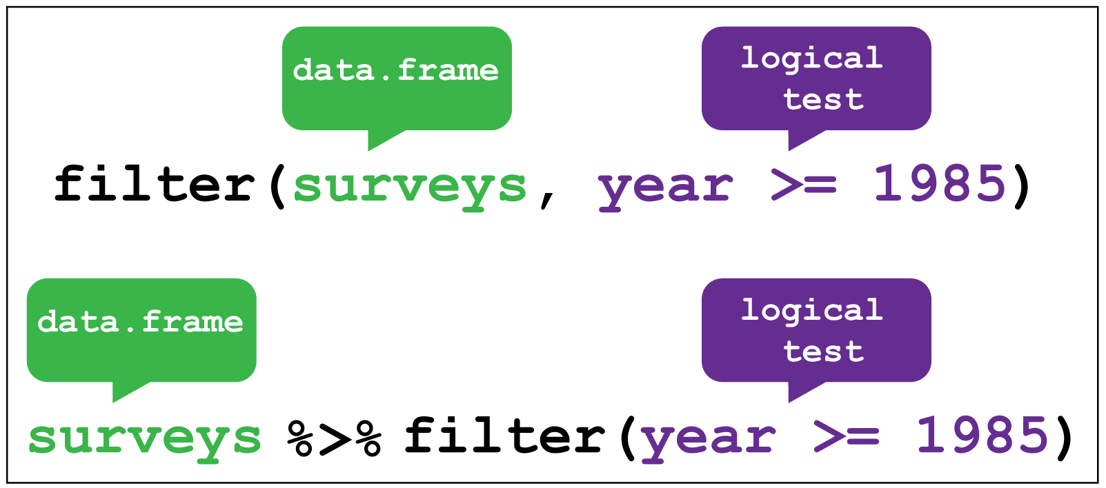
Motivating Example (Pipe Operator)

Use the pipe operator to combine dplyr functions in chain, which allows us to perform more complicated data manipulations

Syntax (Pipe dataframe as input into the dplyr function):

dataframe %>% dplyr_function()

Pipe Example, by Sharp Sight Labs

The pipe operator `%>%`

f(x) %>% g(y) is equivalent to g(f(x),y)

i.e. the output of one function is used as input to the next function. This function can be the identity

Consequences:

x %>% f(y) is the same as f(x,y)
statements of the form k(h(g(f(x,y),z),u),v,w) become x %>% f(y) %>% g(z) %>% h(u) %>% k(v,w)
read %>% as “then do”
in non-mathematical terms, the piping operator allows you to apply more than one different function at the same time to the same data frame.

Filter

Read in the pitch data set. The data are from an experiment on different advanced metrics of MLB baseball pitchers different pitch types.

library(tidyverse)
pitch <- 
  read_csv("https://raw.githubusercontent.com/unl-statistics/R-workshops/main/r-format/data/pitch.csv")

pitch[-1] %>% 
  filter(pitcher_hand == "R", pitch_type == "CU") %>%
  head(n=4)

playerid	pitcher_hand	pitch_type	spin_rate	ab_result	action_result
2795	R	CU	3000.024	\N	F
2795	R	CU	3146.456	\N	B
3646	R	CU	3012.067	\N	B
2795	R	CU	3026.256	HB	B

filter is similar to the base function subset

Filter (cont.)

Multiple conditions in filter are combined with a logical AND (i.e. all conditions must be fulfilled)

e.g.

filter(pitcher_hand == "R", pitch_type == "CU")

Logical expressions can also be used

e.g.

filter(pitcher_hand == "R" & pitch_type == "CU") or filter(pitch_type == "CU" | subject == "KN")

Your Turn (~3 minutes)

Use filter to get a subset of the pitchdata dataset
Ex. Filter the data down to left handed pitchers, who throw a curve with at least 3300 rpms (spin_rate)..
%>% the subset and create a plot

hint: what is the default first argument of the ggplot function?

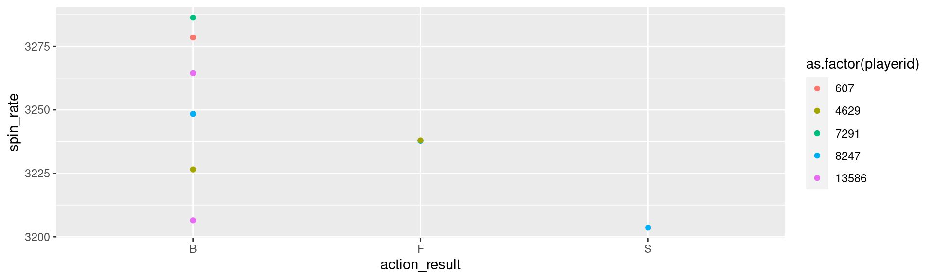
Solution

pitch %>%
  filter(spin_rate >= 3200 & pitcher_hand == "L" & pitch_type == "CU") %>%
  ggplot(aes(x=action_result, y=spin_rate)) +
  geom_point(aes(color=as.factor(playerid)))

Arrange

Easy way to arrange your data in ascending or descending order

pitch %>% 
  subset(select = c("playerid", "spin_rate")) %>%
  arrange(desc(playerid), spin_rate)

playerid	spin_rate
16669	3055.508
16669	3072.307
16669	3075.055
16669	3164.546
15686	3032.944

Arrange

Successive variables are used for breaking ties from previous variables.

pitch %>% 
  subset(select = c("playerid", "spin_rate")) %>%
  arrange(playerid, spin_rate)

playerid	spin_rate
476	3012.770
476	3017.095
476	3024.533
476	3028.328
476	3040.097

Your Turn

Look up the help file for the function slice.
Use slice on the arranged pitchdata dataset to select a single row
use slice to select multiple rows

Hint: Use the entire data set

Solution

pitch[-1] %>% 
  arrange(desc(playerid), spin_rate) %>% 
  slice(11)

playerid	pitcher_hand	pitch_type	spin_rate	ab_result	action_result	adj_h
15540	R	CU	3041.712	\N	F	0

pitch[-1] %>% 
  arrange(desc(playerid), spin_rate) %>% 
  slice(1:5)

playerid	pitcher_hand	pitch_type	spin_rate	ab_result	action_result
16669	R	CU	3055.508	\N	C
16669	R	CU	3072.307	\N	B
16669	R	CU	3075.055	\N	B
16669	R	CU	3164.546	\N	C
15686	R	CU	3032.944	K	S

Select

Using Select we are easily able to create a subset of our data. This is similar to the subset function in base.

pitch %>% 
  select(playerid, pitcher_hand, action_result, spin_rate) %>%
  head()

playerid	pitcher_hand	action_result	spin_rate
2795	R	F	3000.024
959	L	C	3051.596
2795	R	B	3146.456
3646	R	B	3012.067
2795	R	B	3026.256
2795	L	B	3038.633

Summarise

Finding summary statistics of a metric

#na.rm - remove NAs from calculation

pitch %>%
    summarise(mean_spinrate = mean(spin_rate, na.rm=TRUE), 
              sd_spinrate = sd(spin_rate, na.rm = TRUE))

mean_spinrate	sd_spinrate
3125.67	109.8614

`summarise` and `group_by`

Finding summary statistics of a metric after accounting first for other variables

pitch %>%
    group_by(playerid) %>%
    summarise(mean_spinrate = mean(spin_rate, na.rm=TRUE), 
              sd_spinrate = sd(spin_rate, na.rm = TRUE)) %>% 
  head(5)

playerid	mean_spinrate	sd_spinrate
476	3065.601	44.64957
607	3278.486	NA
657	3042.489	43.01146
959	3056.323	42.85757
1030	3044.114	37.69737

Your Turn

Select only playerid, spin_rate, and action result
Group by both playerid and action result and find mean and sd of spin rates
%>% the summaries into a ggplot histogram

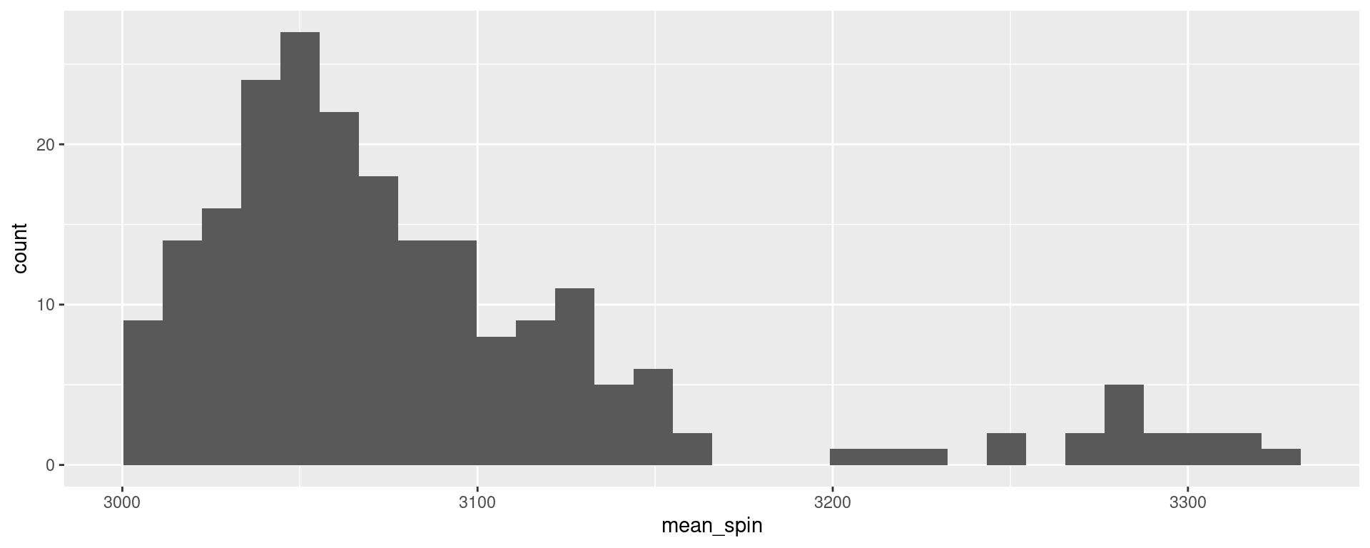
A Solution

pitch %>%
  select(playerid, spin_rate, action_result) %>%
    group_by(playerid, action_result) %>%
    summarise(mean_spin = mean(spin_rate), 
              sd_spin = sd(spin_rate)) %>%
  ggplot(aes(x = mean_spin)) + geom_histogram() #<<

`mutate`

Change an existing or create a new variable into the data
Creating a new column in your data set that represents something new
Great for calculations
How would I create a calculation for how far above or below each players pitches are from their own average spin rates?

`mutate` Example

pitch %>%
    select(playerid, spin_rate, action_result) %>%
    group_by(playerid, action_result) %>%
    summarise(mean_spin = mean(spin_rate), 
              sd_spin = sd(spin_rate)) %>%
    mutate(mean = sum(mean_spin) / n()) %>%
    mutate(difference = mean - mean_spin) %>% head()

# A tibble: 6 × 6
# Groups:   playerid [3]
  playerid action_result mean_spin sd_spin  mean difference
     <dbl> <chr>             <dbl>   <dbl> <dbl>      <dbl>
1      476 B                 3077.   52.1  3058.      -19.1
2      476 F                 3101.    1.69 3058.      -43.4
3      476 S                 3041.   17.0  3058.       17.2
4      476 X                 3013.   NA    3058.       45.3
5      607 B                 3278.   NA    3278.        0  
6      657 B                 3047.   46.2  3036.      -11.2

Utilzing `ifelse`

Sometimes you are tasked to create a new column based on a clause
ifelse function allows you to create an if else statement within the creation of the new variable.
Consider rewriting the handedness of our pitchers.
If the pitcher_hand is R write “Right” if not, “Left”

pitch %>% 
  select(pitcher_hand) %>% 
  mutate(Handedness = ifelse(pitcher_hand == "R", "Right", "Left")) %>% head()

# A tibble: 6 × 2
  pitcher_hand Handedness
  <chr>        <chr>     
1 R            Right     
2 L            Left      
3 R            Right     
4 R            Right     
5 R            Right     
6 L            Left

Caution with pipe operator

Why does pitch$mean_spin not return a real-valued summary??

pitch$mean_spin

NULL

#Columns in our dataset
colnames(pitch[,-1])

[1] "playerid"      "pitcher_hand"  "pitch_type"    "spin_rate"    
[5] "ab_result"     "action_result" "adj_h"

Reasons for pipe operator mishaps

When we use the piping operator like we have been, the data is only ever being changed within the sequence
We only ever look at this new variable in the previous chunk.
It has not been created globally into the dataset itself
To do this, you need to create your new column by declaring it as its own variable.

pitch$mean_spin <- mean(pitch$spin_rate)

`mutate` OR `summarize`?

Both commands introduce new variables - so which one should we use?

mutate

adds variables to the existing data set
The resulting variables must have the same length as the original data
e.g. use for transformations, combinations of multiple variables

summarize

creates aggregates of the original data
The number of rows of the new dataset is determined by the number of combinations of the grouping structure.
The number of columns is determined by the number of grouping variables and the summary statistics.

Shortcuts

summarize(n = n()) is equivalent to tally() (Number of unique rows in dataset)

pitch %>% tally()
pitch %>% summarize(n=n())

Number of unique observations in each group

pitch %>% count(playerid, action_result)
pitch %>% group_by(playerid, action_result) %>% summarize(n=n())
pitch %>% group_by(playerid, action_result) %>% tally()

Your Turn (10 min)

Based on your (limited) knowledge of baseball, you determine what is a “successful” curveball. Then determine what pitchers pitched the most successful curveballs!

Note: There are many different ways of answering this question. None are wrong and you don’t need to know anything about baseball to try. Consider criteria that it needs to meet.

Ex. A successful curveball needs to be above 90 mph in velocity and have over 3100 rpms in spin rate.

utilize the sum() function to add up all your curveballs!

One Solution

Consider a success as any strike (S), catch (C), and foul ball (F)

SScurve <- pitch %>%
  select("playerid", "action_result", "ab_result", "adj_h") %>%  
  arrange(desc(playerid)) %>% 
  mutate(successfulCU = ifelse(
    (action_result %in% c("C","S","F")), 1, 0)) %>%
  group_by(playerid) %>% 
  mutate(totalSSCU=sum(successfulCU)) %>% 
  mutate(percentSSCU=totalSSCU / n())

playerid	action_result	ab_result	successfulCU	totalSSCU	percentSSCU
16669	C	\N	1	2	0.5
16669	B	\N	0	2	0.5
16669	B	\N	0	2	0.5
16669	C	\N	1	2	0.5

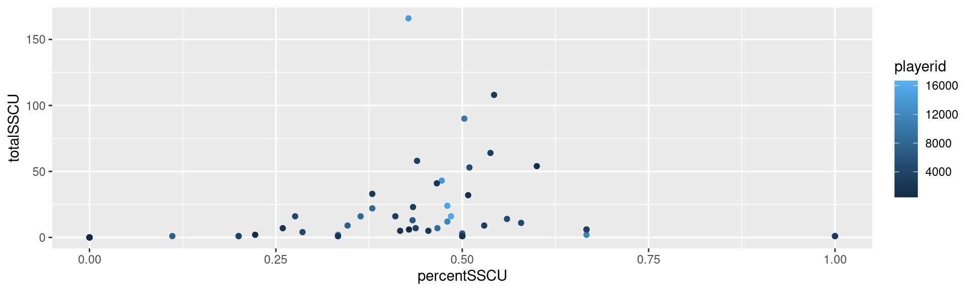
Solution (cont.)

Calculate successful curveball percentages
Look at some graphs to see what the data actually looks like now.

percentages <- SScurve %>% 
  distinct(playerid, totalSSCU, percentSSCU)

ggplot(data = percentages) + 
  geom_point(aes(x = percentSSCU, y = totalSSCU,
                 colour = playerid))

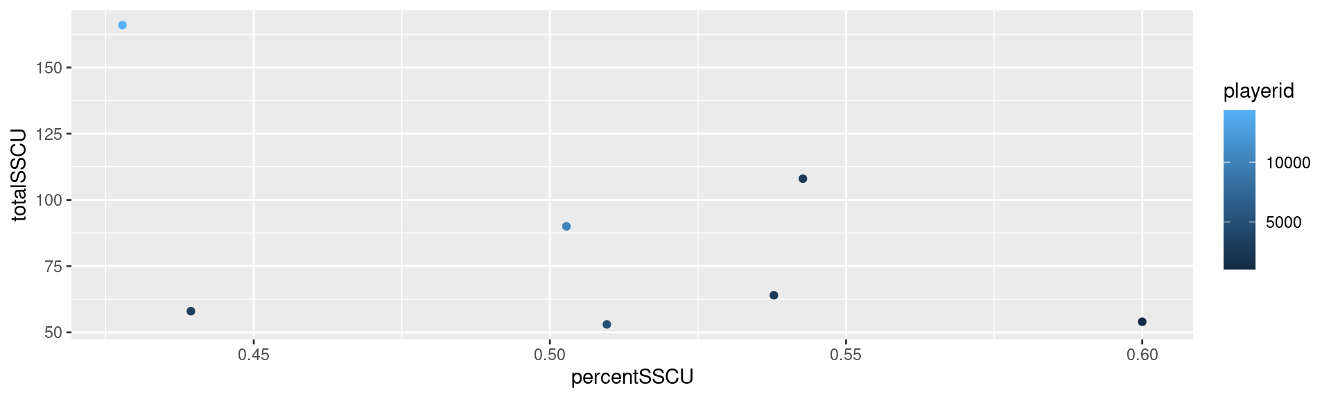
Solution (cont.)

Filter down to get the best pitchers with a minimum of 50 curveballs thrown (our median)

percentages %>% 
  filter(totalSSCU > 50) %>% 
  arrange(desc(percentSSCU)) %>% ggplot() +
   geom_point(aes(x = percentSSCU, y = totalSSCU, colour = playerid))

Your Turn

The dataset ChickWeight is part of the core packages that come with R

Hint: data(ChickWeight) gets the data into your active session.

From the help file:

four groups of chicks on different protein diets. The body weights of the chicks were measured at birth and every second day thereafter until day 20. They were also measured on day 21.

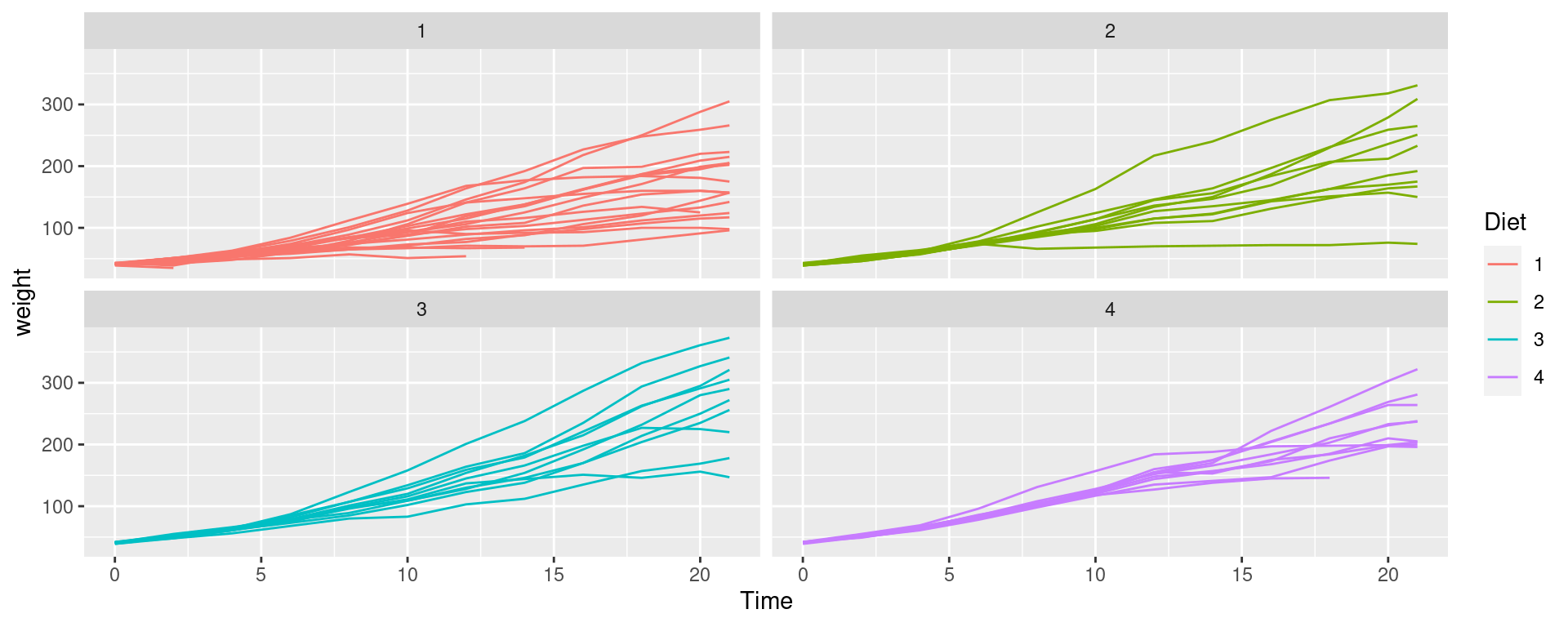
Your Turn

Create a line plot with each line representing the weight of each Chick
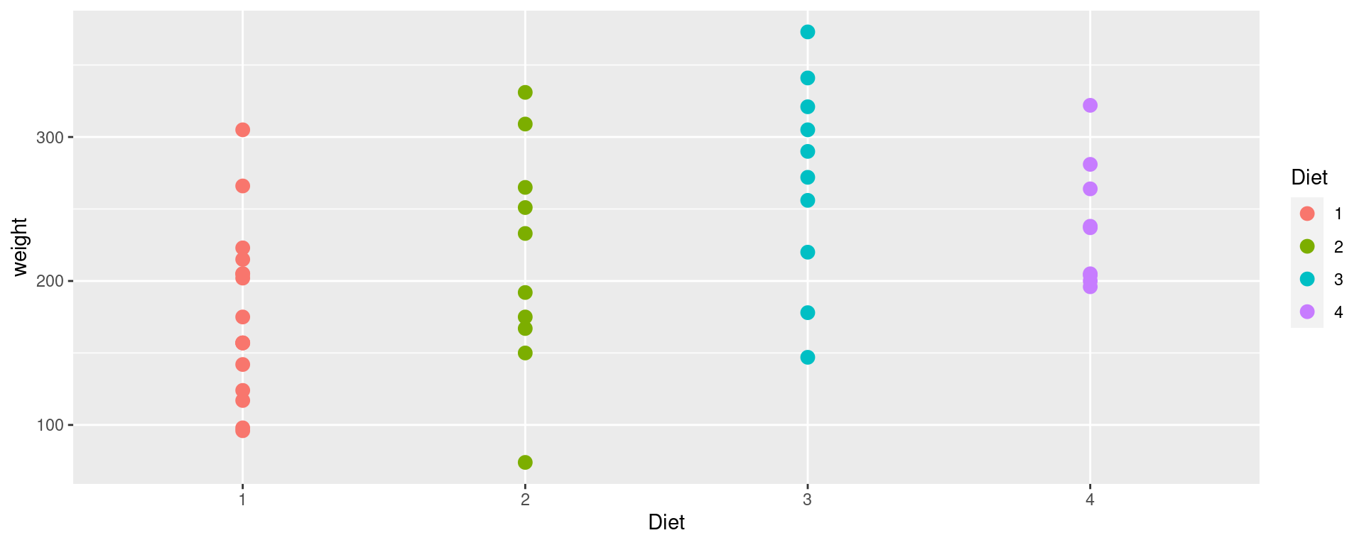
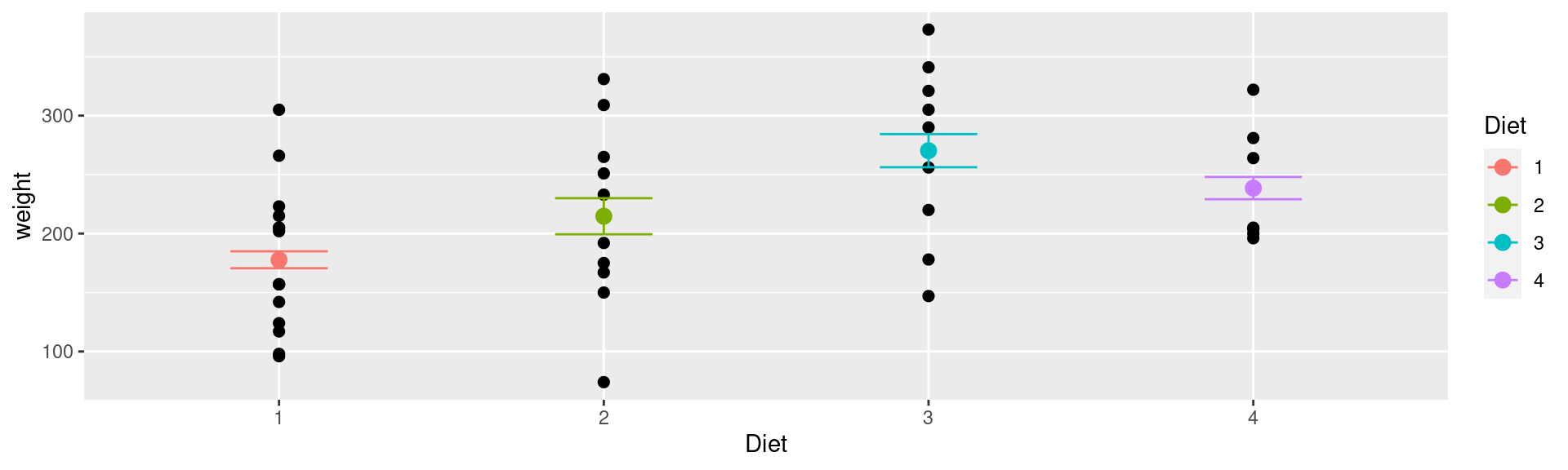
Focus on weight on day 21. Draw side-by-side dotplots of weight by diet.
Bonus: Use summarize the average weight on day 21 under each diet. Overlay the dotplots by error bars around the average weight under each diet (see ?geom_errorbar)

Hint for 1: check out ?group and consider what varible or variables you might map to this option

Solution - Q1

ChickWeight %>% 
  ggplot(aes(x=Time, y=weight, group=Chick, color=Diet)) +
  geom_line() + 
  facet_wrap(~Diet)

Solution - Q2

ChickWeight %>%   
  filter(Time==21) %>% 
  ggplot(aes(x=Diet)) +
  geom_point(aes(y=weight, color=Diet), size=3)

Solution - Q3

First, we need a separate dataset for the summary statistics:

ChickW1 <- ChickWeight %>% 
  filter(Time==21) %>% 
  group_by(Diet) %>% 
  summarize(mean_weight = mean(weight, na.rm=TRUE),
            sd_weight = sd(weight, na.rm=TRUE)/n())

Solution - Q3 (cont)

ChickWeight %>% 
  filter(Time==21) %>% 
  ggplot(aes(x=Diet)) +
  geom_point(aes(y=weight), size=2) +
  geom_errorbar(data= ChickW1, 
                aes(ymin = mean_weight-1.96*sd_weight, 
                    ymax = mean_weight+1.96*sd_weight, 
                    colour = Diet), width=.3) +
  geom_point(data=ChickW1, aes(y=mean_weight, color=Diet), size=3)

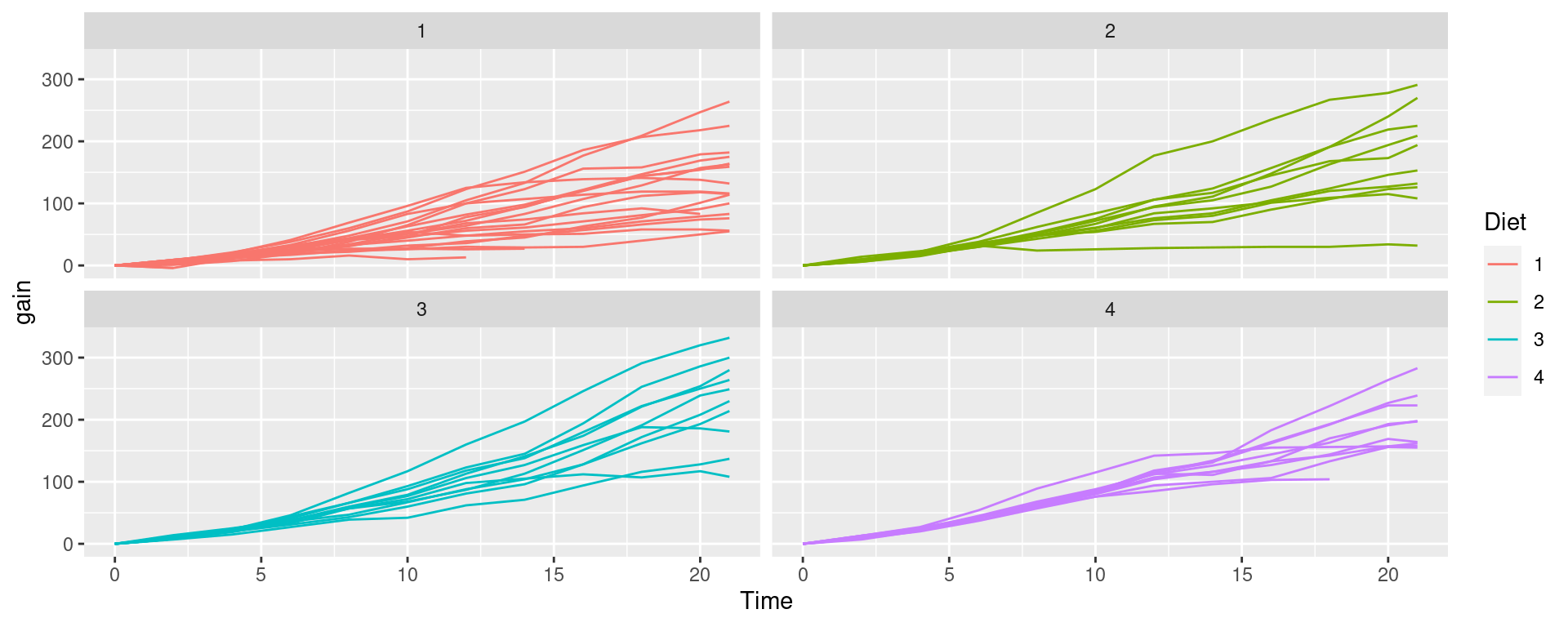
`Mutate` is incredibly flexible

Consider a new variable gain, which gives the increase in weight of a chick since birth

ChickPlus <- ChickWeight %>% 
  group_by(Chick) %>% 
  mutate(gain = weight - weight[Time == 0])

ChickPlus %>% 
  filter(Chick == 1) %>% 
  select(-Diet) %>% 
  glimpse()

Rows: 12
Columns: 4
Groups: Chick [1]
$ weight <dbl> 42, 51, 59, 64, 76, 93, 106, 125, 149, 171, 199, 205
$ Time   <dbl> 0, 2, 4, 6, 8, 10, 12, 14, 16, 18, 20, 21
$ Chick  <ord> 1, 1, 1, 1, 1, 1, 1, 1, 1, 1, 1, 1
$ gain   <dbl> 0, 9, 17, 22, 34, 51, 64, 83, 107, 129, 157, 163

Plotting weight gain

ChickPlus %>% 
  ggplot(aes(x = Time, y = gain, group = Chick)) + 
  geom_line(aes(color=Diet)) +
  facet_wrap(~Diet)

Recap

Getting used to dplyr actions can take a bit of time and practice
Recognize keywords and match them to dplyr functions
Incorporate dplyr functions in your regular workflow - the long-term benefits are there, we promise!

Data Wrangling

dplyr terminology

Motivating Example (Pipe Operator)

The pipe operator %>%

Filter

Filter (cont.)

Your Turn (~3 minutes)

Solution

Arrange

Arrange

Your Turn

Solution

Select

Summarise

summarise and group_by

Your Turn

A Solution

mutate

mutate Example

Utilzing ifelse

Caution with pipe operator

Reasons for pipe operator mishaps

mutate OR summarize?

Shortcuts

Your Turn (10 min)

One Solution

Solution (cont.)

Solution (cont.)

Your Turn

Your Turn

Solution - Q1

Solution - Q2

Solution - Q3

Solution - Q3 (cont)

Mutate is incredibly flexible

Plotting weight gain

Recap

The pipe operator `%>%`

`summarise` and `group_by`

`mutate`

`mutate` Example

Utilzing `ifelse`

`mutate` OR `summarize`?

`Mutate` is incredibly flexible