Simulation Using Built-In Functions

Linear Regression Assumptions

1. Linearity and Additivity of DVs

2. Independence of Errors

3. Constant Variance of Errors

4. Normality of Errors

How Bad is it? – Linearity

library(tidyverse)
set.seed(2034927344)
data <- tibble(
  x1 = seq(-10, 10, 
           length.out = 100) + 
    runif(100, -.1, .1), # wiggle
  x2 = seq(10, -10, 
           length.out = 100) + 
    runif(100, -.1, .1), # wiggle
  
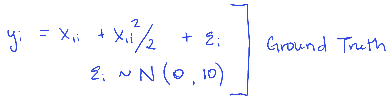
  # Definitely not linear
  y =  x1 + x1^2/2 + # main effect
    rnorm(100, 0, 10) # actual error
)

ggplot(data, aes(x = x1, y = y)) + 
  geom_point()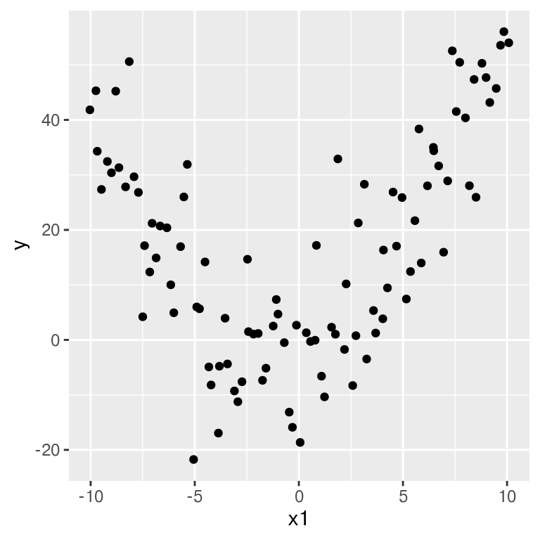

Clearly non-linear

How Bad is it? – Linearity

model <- lm(y ~ x1 + x2, data = data)
summary(model)

Call:
lm(formula = y ~ x1 + x2, data = data)

Residuals:
    Min      1Q  Median      3Q     Max 
-35.805 -15.641  -1.853  16.714  44.165 

Coefficients:
            Estimate Std. Error t value Pr(>|t|)    
(Intercept)   16.457      1.913   8.605 1.37e-13 ***
x1           -20.473     24.200  -0.846    0.400    
x2           -21.413     24.238  -0.883    0.379    
---
Signif. codes:  0 '***' 0.001 '**' 0.01 '*' 0.05 '.' 0.1 ' ' 1

Residual standard error: 19.08 on 97 degrees of freedom
Multiple R-squared:  0.07991,   Adjusted R-squared:  0.06094 
F-statistic: 4.212 on 2 and 97 DF,  p-value: 0.01761

How Bad is it?

model2 <- lm(y ~ x1 + I(x1^2), data = data)
summary(model2)

Call:
lm(formula = y ~ x1 + I(x1^2), data = data)

Residuals:
     Min       1Q   Median       3Q      Max 
-29.1382  -6.9539  -0.2898   5.4694  30.6999 

Coefficients:
            Estimate Std. Error t value Pr(>|t|)    
(Intercept) -1.30483    1.55887  -0.837    0.405    
x1           0.90094    0.17844   5.049 2.08e-06 ***
I(x1^2)      0.51842    0.03407  15.214  < 2e-16 ***
---
Signif. codes:  0 '***' 0.001 '**' 0.01 '*' 0.05 '.' 0.1 ' ' 1

Residual standard error: 10.41 on 97 degrees of freedom
Multiple R-squared:  0.7261,    Adjusted R-squared:  0.7205 
F-statistic: 128.6 on 2 and 97 DF,  p-value: < 2.2e-16

Models

Simulation – Questions

1. How does \(\hat{s}\) compare to \(\sigma=10\)?
2. How does \(\hat\alpha\) compare to true value \(\alpha=1\)?
3. How does \(\hat\beta\) compare to true value \(\beta=0\)?

Simulation – Linearity assumption

sim_linearity <- function(i, n = 100, formula = y ~ x1+x2, trueformula = y ~ x1 + I(x1^2)) {
  data <- tibble(
    x1 = seq(-10, 10, length.out = n) + runif(n, -.1, .1),
    x2 = seq(-10, 10, length.out = n) + runif(n, -.1, .1),
    y =  x1 + x1^2/2 + rnorm(n, 0, 10) # Definitely not additive or linear
  )
  
  model <- lm(formula = formula, data = data)
  model2 <- lm(formula = trueformula, data = data)
  tibble(
    i = i, 
    data = list(data), 
    model = tibble(type = c("misspec", "actual"), 
                   model = list(model, model2))
         )
}

set.seed(249382736)
sim_n <- map_df(1:1000, ~sim_linearity(.)) |> 
  unnest(model)

Simulation – Getting Estimates Out

library(broom) # very useful for tidying nested model dataframes

sim_n <- sim_n |> mutate(
  # One line per parameter
  tidy_model = purrr::map(model, tidy), 
  # One line per model
  glance_model = purrr::map(model, glance))  

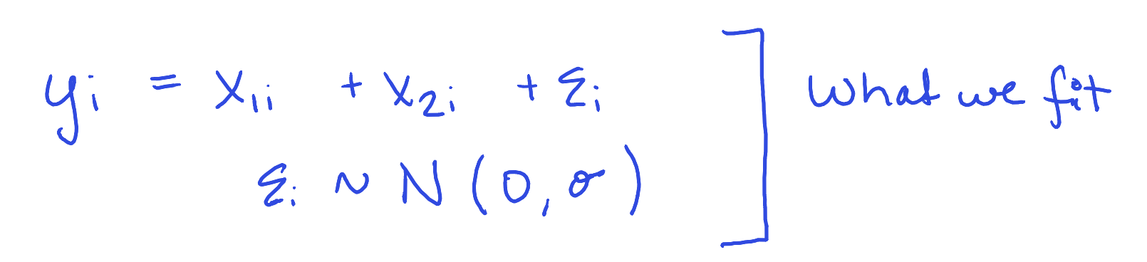
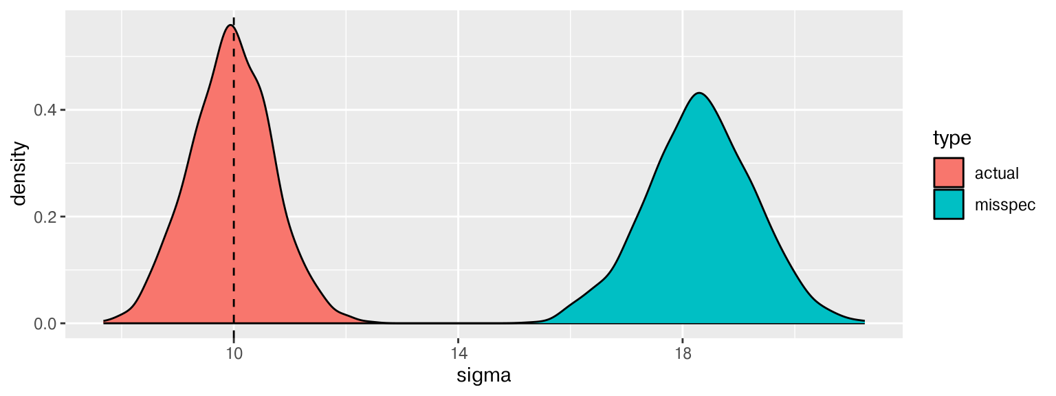
Error Variance

tmp <- sim_n |>
  unnest(glance_model)
ggplot(tmp, aes(x = sigma, fill = type)) + 
  geom_density() + 
  geom_vline(xintercept = 10, linetype = "dashed")

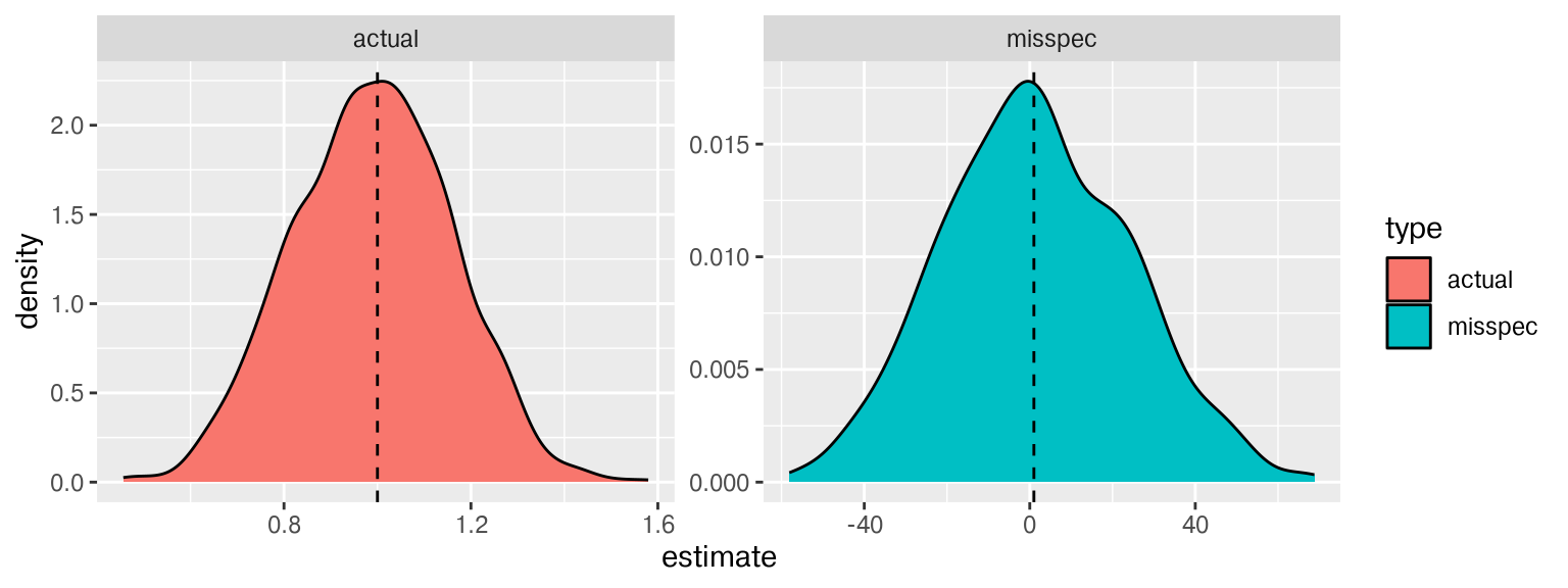
\(\alpha\) coefficient

sim_n|>
  unnest(tidy_model) |> filter(term == "x1") |>
  ggplot(aes(x = estimate, fill = type)) + 
  geom_density() + 
  geom_vline(xintercept = 1, linetype = "dashed") + 
  facet_wrap(~type, scales="free")

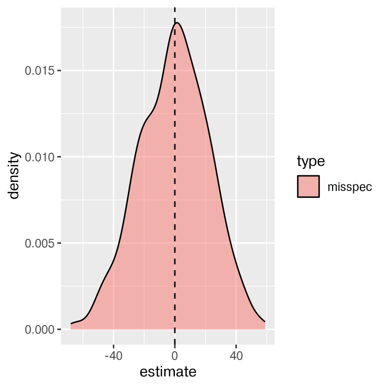
That is some wide error variance!

\(\beta\) coefficient

sim_n|>
  unnest(tidy_model) |>
  # Only occurs in misspec model
  filter(term == "x2") |>
  ggplot(aes(x = estimate, fill = type)) + 
  geom_density(alpha=0.5) + 
  geom_vline(xintercept = 0, 
             linetype = "dashed")